Estimating a Bayesian VAR

Jörg Rieger

17 7 2019

Introduction

The purpose of this vignette is to show how to estimate Bayesian Vector Autoregressive Models using the package bvar2.

We do this by using a

The model is estimated in 2 steps:

• Define the prior for the model
• Estimate the bayesian VAR-model using the above defined prior

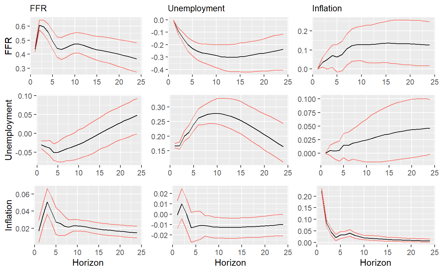
We can use an estimated model to compute impulse-response functions or make forecasts. Here, we will compute impulse-response functions from an estimated model.

Setting up the prior

In the first step, we set up the prior. For the simplest case we use an uninformative prior.

While the uninformative prior itself has (as the name says) no prior information about the parameters we aim to estimate. We still have to provide the creator function with some information about the model. These information are

• The number of lags of the model
• Whether the model has an intercept or not

In addition, we have to provide the data to estimate the parameters. The function uses the data to extract some basic information, such as the number of variables, of it.

library(bvars)
data("USMonPol")
prior <- set_prior_uninformative(mydata = USMonPol,nolags = 6, intercept = TRUE)

Estimating a Bayesian VAR model

Having created the prior we now estimate a bvar model.

bvestimate <- bvars::bvar(mydata=USMonPol,priorObj = prior,
                          stabletest = T,nthin = 2,
                          nreps = 1100, burnin = 100)

## Initialize MCMC sampler for uninformative prior
## draw no. 1000

Computing and plotting Impulse-Response Functions

Impulse-Response Functions are an

id <- set_identification_cholesky()
bvirf <- bvars::irf(bvestimate,id,nhor=24)
plot(bvirf)